MLF Lecture 5 Training versus Testing
機器學習基石(Machine Learning Foundations)笔记第五弹
Theory of Machine Learning can be split into Two Central Question
\[\begin{aligned} \color{green}{\large\text{Two Central Question}} \end{aligned}\] \[\begin{aligned} & \text{for }\underbrace{\text{batch & supervised binary classification}}_{lecture 3}, \color{purple}{\underbrace{g \simeq f}_{ \text{lecture 1}} \Longleftrightarrow E_{out}(g) \simeq 0} \\\ & \text{achieved through} \color{orangered}{\underbrace{E_{out}(g) \simeq E_{in}(g)}_{ \text{lecture 4}}} \text{ and } \color{crimson}{\underbrace{E_{in}(g) \simeq 0}_{ \text{lecture 2}}} \end{aligned}\]hieved through} \end{aligned}
所以机器学习的目的研究方向主要分为两部分:
- 保证 \(E_{out}(g)\) 与 \(E_{in}(g)\) 很接近
- 尽量减小 \(E_{in}(g)\)
其中 \(\color{blue}{\underbrace{M}_{|H|}}\) 是研究两个问题的关键之一
When it comes to infinite hypothesis set
Known
\[\begin{aligned} \mathbb{P}[\mid E_{in}(h) - E_{out}(h)\mid > \epsilon] \leq 2 exp(-2\epsilon^2N) \end{aligned}\]Todo
- establish \(\color{orangered}{\text{a finite quantity}}\) that replaces \(\color{orangered}{M}\)
- justify the feasibility of learning for infinite M
- study \(\color{orangered}{m_h}\) to understand its trade off for 'right' \(\mathcal H\) , just like M
我们希望能将 infinite 的 M 换成一个与 Hypothesis 有关的 \(\bf{m_h}\) ,控制不等号右边上界的范围
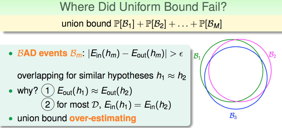
Overestimation of Union Bound
在计算 \(\mathbb P \left[|E_{in}(g) - E_{out}(g)| > \epsilon \right]\) 时(我将其称为 \(E_{in}(g)\) 与 \(E_{out}(g)\) 的偏离概率),我们进行了放缩:
\[\begin{aligned} \mathbb P [B_1\ or B_2\ or \dots B_M]\color{orangered}{\underbrace{\leq}_{union\ bound}} \mathbb P [B_1] + \mathbb P[B_2] + \dots \mathbb P [B_M] \end{aligned}\]然而实际情况是,由于 Hypothesis 中由许多极其相似的 h,所以每个 Bad Data 代表的范围有很大一部分是重合的,所以我们在使用 union bound 放缩时,
把重叠的主要部分都算进去了,导致对上界的过度估计。
Effective Line Numbers
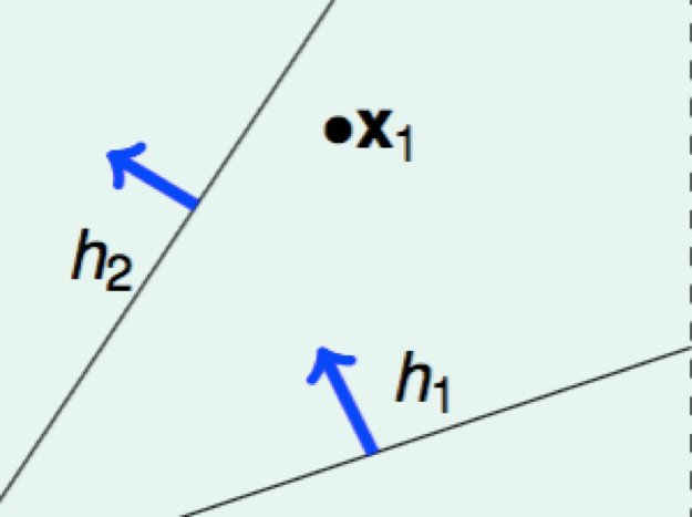
我们先研究在二维平面内,对数据 \(x_1,x_2,\dots x_n\) 来说,有效的线段(effectice lines)有哪几种。
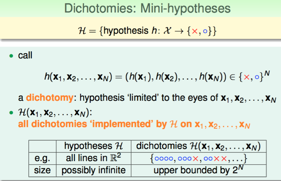
Effective Lines: 将数据分成 Ο 或 X 的线,划分后数据状况一样的线都是同一种 Effective Line
- N = 1: 2 kinds
N = 2: 4 kinds
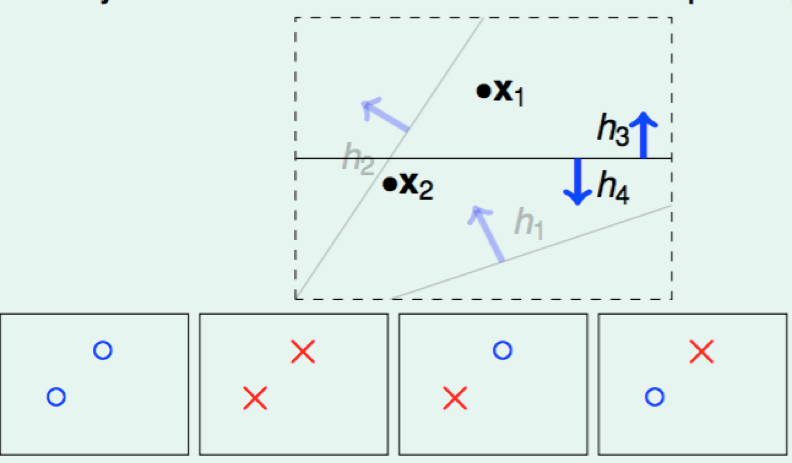
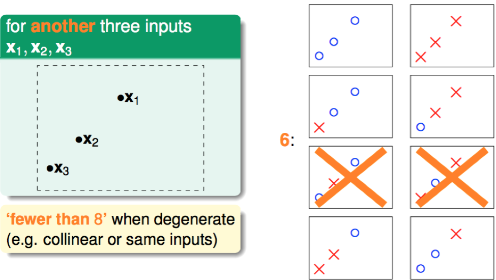
N = 3: max 8 kinds
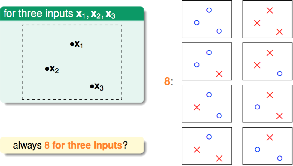
三点共线: only 6 kinds
N = 4: max 14 kinds
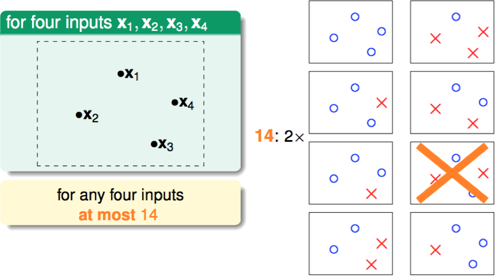
容易看出,对于 N 个数据,最多 \(2^N\) 种 Effective Lines(每个点的状态均有两种)
PS: 二维平面上 Kinds of Effective Lines
数法:分别输出 1 个相邻的点同状态,2 个相邻的点状态,... N 个相邻的点同状态的种数,然后相加。
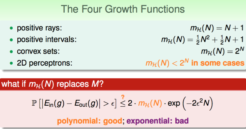
因此,我们希望能够用关于 N 的成长函数(growth function)来取代 Hypothesis 的数量 M,当 effective(N)增长足够慢时且 N 很大时,即:
\[\begin{aligned} \mathbb P[|E_{in}(g) - E{out}(g)| > \epsilon] \leq 2 \cdot \color{orangered}{effective(N)} \cdot exp(-2\epsilon^2N) \quad (effective(N) \ll 2^N) \end{aligned}\]\(E_{in}\) 与 \(E_{out}\) 的偏离概率足够小,从而使 Machine Learning 可能。
Dichotomy(二分法)
Growth Function
定义:数据量为 N 的所有数据情况中 Hypothesis 种类数量最多 \(\large m_h(N)\) 最大的函数
含义:为了摆脱 \(\large m_h(N)\) 对一定数据量 N 下数据不同排列组合情况的依赖
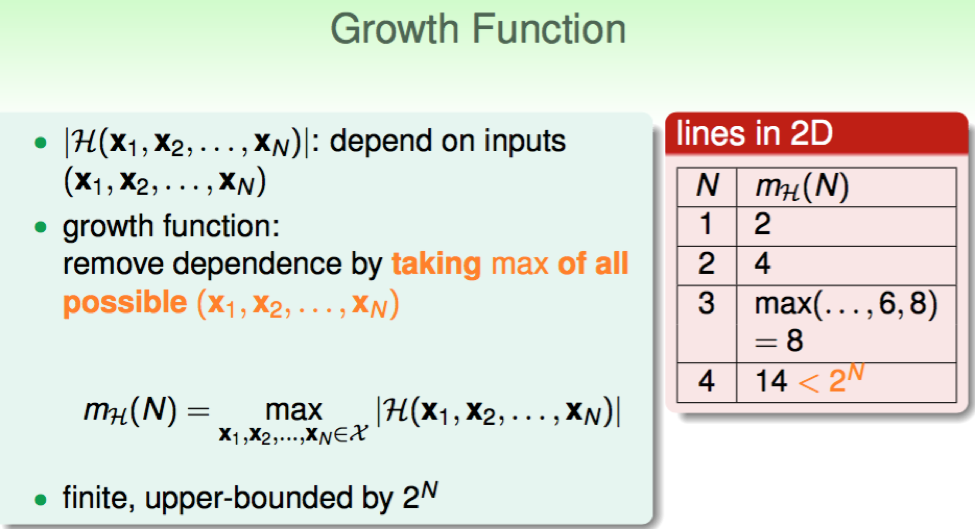
关于四种情况下增长函数的详细内容参见第五章课件
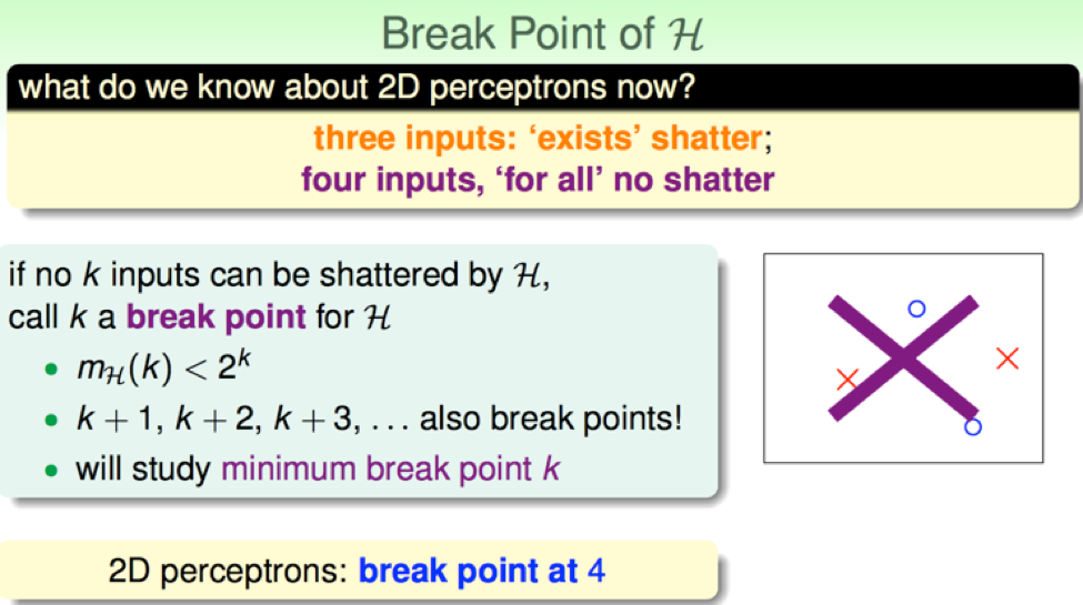
Break Point
shatter: Hypothesis 种类 = 2N 的情况
Break Point(突破点): 使得当前数据无法出现 shatter 的 N 的值
比如二维的 perceptrons 下,N = 4 时 Hypothesis 种类最多为 14 < 24